4 A Tidy Framework and Infrastructure to Systematically Assemble Spatio-temporal Indexes from Multivariate Data
Indexes are useful for summarizing multivariate information into single metrics for monitoring, communicating, and decision-making. While most work has focused on defining new indexes for specific purposes, more attention needs to be directed towards making it possible to understand index behavior in different data conditions, and to determine how their structure affects their values and variation in values. Here we discuss a modular data pipeline recommendation to assemble indexes. It is universally applicable to index computation and allows investigation of index behavior as part of the development procedure. One can compute indexes with different parameter choices, adjust steps in the index definition by adding, removing, and swapping them to experiment with various index designs, calculate uncertainty measures, and assess indexes’ robustness. The paper presents three examples to illustrate the pipeline framework usage: comparison of two different indexes designed to monitor the spatio-temporal distribution of drought in Queensland, Australia; the effect of dimension reduction choices on the Global Gender Gap Index (GGGI) on countries’ ranking; and how to calculate bootstrap confidence intervals for the Standardized Precipitation Index (SPI). The methods are supported by a new R package, called tidyindex.
4.1 Introduction
Indexes are commonly used to combine and summarize different sources of information into a single number for monitoring, communicating, and decision-making. They serve as critical tools across the natural and social sciences. Examples include the Air Quality Index, El Niño-Southern Oscillation Index, Consumer Price Index, QS University Rankings, and the Human Development Index. In environmental science, climate indexes are produced by major monitoring centers, like the United States Drought Monitor and National Oceanic and Atmospheric Administration, to facilitate agricultural planning and early detection of natural disasters. In economics, indexes provide insight into market trends through combining prices of a basket of goods and services. In social sciences, indexes are used to monitor human development, gender equity, or university quality. The problem is that every index is developed in its own unique way, by different researchers or organizations, and often indexes designed for the same purpose cannot easily be compared.
To construct an index, experts typically start by defining a concept of interest that requires measurement. This concept often lacks a direct measurable attribute or can only be measured as a composite of various processes, yet it holds social and public significance. To create an index, once the underlying processes involved are identified, relevant and available variables are then defined, collected, and combined using statistical methods into an index that aims to measure the process of interest. The construction process is often not straightforward, and decisions need to be made, such as the selection of variables to be included, which might depend on data availability and the statistical definition of the index to be used, among others. For instance, the indexes constructed from a linear combination of variables require to decide the weight assigned to each variable. Some indexes have a spatial and/or temporal component, and variables can be aggregated to different spatial resolutions and temporal scales, leading to various indexes for different monitoring purposes. Hence, all these decisions can result in different index values and have different practical implications.
To be able to test different decision choices systematically for an index, the index needs to be broken down into its fundamental building blocks to analyze the contribution and effect of each component. We call this process of breaking the index construction into different steps the index pipeline. Such decomposition of index components provides the means to standardize index construction via a pipeline and offers benefits for comparing among indexes, calculating index uncertainty, and assessing index robustness.
In this work, we provide statistical and computational methods for developing a data pipeline framework to construct and customize indexes using data. The proposed pipeline comprises various modules, including temporal and spatial aggregation, variable transformation and combination, distribution fitting, benchmark setting, and index communication. Given the decisions analysts need to make when combining multivariate data into indexes, the proposed pipeline enables the evaluation of how the specific choice can affect the index, as well as how the index may appear under alternative options. Furthermore, uncertainty calculation can also flow through the pipeline, providing the index with confidence measures.
The rest of the paper is structured as follows. Section 4.2 provides background about the development of indexes. Section 4.3 reviews the tidy framework in R and how index construction can benefit from such a framework. The details of the pipeline modules are presented in Section 4.4. Section 4.5 explains the design of the tidyindex package that implements the modules. Examples are given in Section 4.6 to illustrate three use cases of the pipeline.
4.2 Background to index development
There are many documents providing advice on how to construct indexes for different fields, and review articles describing the range of available indexes for specific purposes. The OECD handbook (OECD, European Union, and Joint Research Centre - European Commission 2008) provides a comprehensive guide for computing socio-economic composite indexes, with detailed steps and recommendations. The drought index handbook (Svoboda, Fuchs, et al. 2016) provides details of various drought indexes and recommendations from the World Meteorology Organization. Zargar et al. (2011), Hao and Singh (2015) and Alahacoon and Edirisinghe (2022) are review papers describing the range of possible drought indexes.
There is also some attention being given to the diagnosis of indexes, and incorporation of uncertainty. Jones and Andrey (2007) investigates the methodological choices made in the development of indexes for assessing vulnerable neighborhoods. Saisana, Saltelli, and Tarantola (2005) describes incorporating uncertainty estimates and conducting sensitivity analysis on composite indexes. Tate (2012) and Tate (2013), similarly, make a comparative assessment of social vulnerability indexes based on uncertainty estimation and sensitivity analysis. Laimighofer and Laaha (2022) studies five uncertainty sources (record length, observation period, distribution choice, parameter estimation method, and GOF-test) of drought indexes.
There are also a few R packages supporting index calculation. The SPEI package (Vicente-Serrano, Beguería, and López-Moreno 2010) computes two drought indexes. The gpindex package (Martin 2023) computes price indexes, and the fundiversity package (Grenié and Gruson 2023) computes functional diversity indexes for ecological study. The package COINr (Becker et al. 2022) is more ambitious, making a start on following the broader guidelines in the OECD handbook to construct, analyze, and visualize composite indexes.
From reviewing this literature, and in the process of developing methods for making it easier to work with multivariate spatio-temporal data, it seems possible to think about indexes in a more organised, cohesive and standard manner. Actually, the area could benefit from a tidy approach.
4.3 Tidy framework
The tidy framework consists of two key components: tidy data and tidy tools. The concept of tidy data (Wickham 2014) prescribes specific rules for organizing data in an analysis, with observations as rows, variables as columns, and types of observational units as tables. Tidy tools, on the other hand, are concatenated in a sequence through which the tidy data flows, creating a pipeline for data processing and modeling. These pipelines are data-centric, meaning all the tidy tools or functions take a tidy data object as input and return a processed tidy data object, directly ready for the next operations to be applied. Also, the pipeline approach corresponds to the modular programming practice, which breaks down complex problems into smaller and more manageable pieces, as opposed to a monolithic design, where all the steps are predetermined and integrated into a single piece. The flexibility provided by the modularity makes it easier to modify certain steps in the pipeline and to maintain and extend the code base.
Examples of using a pipeline approach for data analysis can be traced back to the interactive graphics literature, including Buja et al. (1988); Sutherland et al. (2000); Wickham et al. (2009); Xie, Hofmann, and Cheng (2014). Wickham et al. (2009) argue that whether made explicit or not, a pipeline has to be presented in every graphics program, and making them explicit is beneficial for understanding the implementation and comparing between different graphic systems. While this comment is made in the context of interactive graphics programs, it is also applicable generally to any data analysis workflow. More recently, the tidyverse suite (Wickham et al. 2019) takes the pipeline approach for general-purpose data wrangling and has gained popularity within the R community. The pipeline-style code can be directly read as a series of operations applied successively on tidy data objects, offering a method to document the data wrangling process with all the computational details for reproducibility.
Since the success of tidyverse, more packages have been developed to analyze data using the tidy framework for domains specific applications, a noticeable example of which is tidymodels for building machine learning models (Kuhn and Wickham 2020). To create a tidy workflow tailored to a specific domain, developers first need to identify the fundamental building blocks to create a workflow. These components are then implemented as modules, which can be combined to form the pipeline. For example, in supervised machine learning models, steps such as data splitting, model training, and model evaluation are commonly used in most workflow. In the tidymodels, these steps are correspondingly implemented as package rsample, parsnip, and yardstick, agnostic to the specific model chosen. The uniform interface in tidymodels frees analysts from recalling model-specific syntax for performing the same operation across different models, increasing the efficiency to work with different models simultaneously.
For constructing indexes, the pipeline approach adopts explicit and standalone modules that can be assembled in different ways. Index developers can choose the appropriate modules and arrange them accordingly to generate the data pipeline that is needed for their purpose. The pipeline approach provides many advantages:
- makes the computation more transparent, and thus more easily debugged.
- allows for rapidly processing new data to check how different features, like outliers, might affect the index value.
- provides the capacity to measure uncertainty by computing confidence intervals from multiple samples as generated by bootstrapping to original data.
- enables systematic comparison of surrogate indexes designed to measure the same phenomenon.
- it may even be possible to automate diagrammatic explanations and documentation of the index.
Adoption of this pipeline approach would provide uniformity to the field of index development, research, and application to improve comparability, reproducibility, and communication.
4.4 Details of the index pipeline
In constructing various indexes, the primary aim is to transform the data, often multivariate, into a univariate index. Spatial and temporal considerations are also factored into the process when observational units and time periods are not independent. However, despite the variations in contextual information for indexes in different fields, the underlying statistical methodology remains consistent across diverse domains. Each index can be represented as a series of modular statistical operations on the data. This allows us to decompose the index construction process into a unified pipeline workflow with a standardized set of data processing steps to be applied across different indexes.
An overview of the pipeline is presented in ?fig-pipeline-steps, illustrating the nine available modules designed to obtain the index from the data. These modules include operations for temporal and spatial aggregation, variable transformation and combination, distribution fitting, benchmark setting, and index communication. Analysts have the flexibility to construct indexes by connecting modules according to their preferences.
Now, we introduce the notation used for describing pipeline modules. Consider a multivariate spatio-temporal process,
\begin{equation} \mathbf{x}(s;t) = \{x_1(s;t), x_2(s;t), \cdots, x_p(s;t)\} \qquad s \in D_s \subseteq \mathbb{R}^m, t \in D_t \subseteq \mathbb{R}^n \end{equation}where:
x_j(s, t) represents a variable of interest for example precipitation, j = 1, \cdots, p and
s represents the geographic locations in the space D_s \subseteq \mathbb{R}^m. Examples of geographic locations include a collection of countries, longitude and latitude coordinates or regions of interest and,
t denotes the temporal order in D_t \subseteq \mathbb{R}^n. For instance, time measurements could be recorded hourly, yearly, monthly, quarterly, or by season.
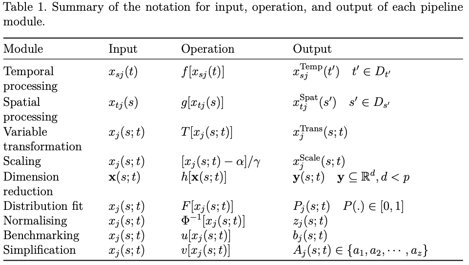
In what follows when geographic or temporal components of the x_j(s,t) process are fixed we will be using suffix notation. For example, x_{sj}(t) represents the data for a fixed location s as a function of time t. While x_{tj}(s) denotes the spatial varying process for a fixed t. An overview of the notation for pipeline input, operation, and output is present in Table 1:
Temporal processing
The temporal processing module takes as input argument a single variable x_{sj}(t) at location s as a function of time. In this step the original time series can be transformed or summarized into a new one via time aggregation, the transformation is represented by the function f, x^{\text{Temp}}_{sj}(t^\prime) = f[x_{sj}(t)] where t^\prime refers to the new temporal resolution after aggregation. An example of temporal processing done in the computation of the Standardized Precipitation Index (SPI) (McKee et al. 1993), consists of summing the monthly precipitation series over a rolling time window of size k. That is also known as the time scale. For SPI, the choice of the time scale k is used to control the accumulation period for the water deficit, enabling the assessment of drought severity across various types (meteorological, agricultural, and hydrological).
Spatial processing
The spatial processing module takes a single variable with a fixed temporal dimension, x_{tj}(s), as input. This step transforms the variable from the original spatial dimension s into the new dimension s^\prime \in D_{s^\prime} through x^{\text{Spat}}_{tj}(s^\prime) = g[x_{tj}(s)]. The change of spatial dimension allows for the alignment of variables collected from different measurements, such as in-situ stations and satellite imagery, or originating from different resolutions. This also includes the aggregation of variables into different levels, such as city, state, and country scales.
Variable transformation
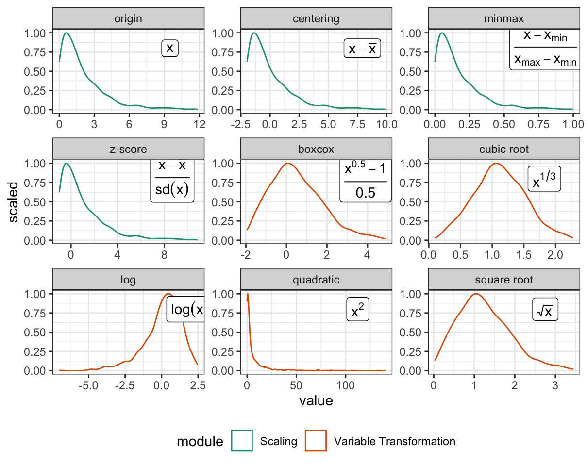
Variable transformation takes the input of a single variable x_j(s;t) and reshapes its distribution using the function T[.] to produce x^{\text{Trans}}_{j}(s;t). When a variable has a skewed distribution, transformations such as log, square root, or cubic root can adjust the distribution towards normality. For example, in the Human Development Index (HDI), a logarithmic transformation is applied to the variable Gross National Income per capita (GNI), to reduce its impact on HDI, particularly for countries with high GNI values.
Scaling
Unlike variable transformation, scaling maintains the distributional shape of the variable. It includes techniques such as centering, z-score standardization, and min-max standardization and can be expressed as [x_{j}(s;t) - \alpha]/\gamma. In the Human Development Index (HDI), the three dimensions (health, education, and economy) are converted into the same scale (0-1) using min-max standardization.
Although the scaling might be considered to be a transformation, we have elected to make it a separate module because it is neater. Scaling simply changes the numbers in the data not the shape of a variable. Transformation will most likely change the shape, and is usually non-linear.
Dimension reduction
Dimension reduction takes the multivariate information \mathbf{x}(s;t), where \mathbf{x} \subseteq \mathbb{R}^p, or a subset of variables in \mathbf{x}(s;t), as the input. It summarises the high-dimensional information into a lower-dimension representation \mathbf{y}(s;t), where y \subseteq \mathbb{R}^d and d < p, as the output. The transformation can be based on domain-specific knowledge, originating from theories describing the underlying physical processes, or guided by statistical methods. For example, the Standardized Precipitation-Evapotranspiration Index (SPEI) (Beguería and Vicente-Serrano 2017) calculates the difference D between precipitation (P) and potential evapotranspiration (\text{PET}), using a water balance model (D = P - \text{PET}). This is the only step that differs from the Standardized Precipitation Index (SPI), and can be considered to be a dimension reduction using a particular linear combination.
Linear combinations of variables are commonly used to reduce the dimension in statistical methodology, and chosen using a method like principal component analysis (PCA) (Hotelling 1933) or linear discriminant analysis (Fisher 1936), preparing contrasts to test particular elements in analysis of variance (Fisher 1970), or hand-crafted by a content-area expert. Linear combinations also form the basis for visualizing multivariate data, in methods such as tours (Wickham et al. 2011). This dimension reduction method can accommodate linear combinations as provided by any method, and hence is linear by design. The transformation module provides variable-wise non-linear transformation.
Distribution fit
Distribution fit applies the Cumulative Distribution Function (CDF) F of a distribution on the variable x_j(s; t) to obtain the probability values P_j(s;t) \in [0, 1]. In SPEI, many distributions, including log-logistic, Pearson III, lognormal, and general extreme distribution, are candidates for the aggregated series. Different fitting methods and different goodness of fit tests may be used to compare the distribution choice on the index value. This could be considered to be a variable transformation because it is usually conducted separately for each variable. However, very occasionally a fit is conducted on two or more variables simultaneously. For this reason, and because it usually is applied later in the pipeline it is neater to make this a separate module.
Normalising
Normalizing applies the inverse normal CDF \Phi^{-1} on the input data to obtain the normal density z_{j}(s;t). Normalizing can sometimes be confused with the scaling or variable transformation module, which does not involve using a normal distribution to transform the variable. It is arguably whether normalizing and distribution fit should be combined or separated into two modules. A decision has been made to separate them into two modules given the different types of output each module presents (probability values for distribution fit and normal density values for normalizing).
Benchmarking
Benchmark sets a value b_j(s,t) for comparing against the original variable x_j(s;t). This benchmark can be a fixed value consistently across space and time or determined by the data through the function u[x_j(s;t)]. Once a benchmark is set, observations can be highlighted for adjustments in other modules or can serve as targets for monitoring and planning.
Simplification
Simplification takes a continuous variable x_j(s;t) and categorises it into a discrete set A_j(s;t) \in \{a_1, a_2, \cdots, a_z\} through a piecewise constant function,
\begin{equation} v[x_i(s;t)] = \begin{cases} a_0 & C_1 \leq x^i(s; t) < C_0 \\ a_1 & C_2 \leq x^i(s; t) < C_1 \\ a_2 & C_3 \leq x^i(s; t) < C_2 \\ \cdots \\ a_z & C_z \leq x^i(s; t) \end{cases} \end{equation}This is typically used at the end of the index pipeline to simplify the index to communicate to the public the severity of the concept of interest measured by the index. An example of simplification is to map the calculated SPI to four categories: mild, moderate, severe, and extreme drought.
4.5 Software design
The R package tidyindex implements a proof-of-concept of the index pipeline modules described in Section 4.4. These modules compute an index in a sequential manner, as shown below:
DATA |>
  module1(...) |>
  module2(...) |>
  module3(...) |>
  ...
Each module offers a variety of alternatives, each represented by a distinct function. For example, within the dimension_reduction() module, three methods are available: aggregate_linear(), aggregate_geometrical(), and manual_input() and they can be used as:
dimension_reduction(V1 = aggregate_linear(...))
dimension_reduction(V2 = aggregate_geometrical(...))
dimension_reduction(V3 = manual_input(...))
Each method can be independently evaluated as a recipe, for example,
manual_input(~x1 + x2)takes a formula to combine the variables x1 and x2 and return:
[1] "manual_input"
attr(,"formula")
[1] "x1 + x2"
attr(,"class")
[1] "dim_red"
This recipe will then be evaluated in the pipeline module with data to obtain numerical results. The package also offers wrapper functions that combine multiple steps for specific indexes. For instance, the idx_spi() function bundles three steps (temporal aggregation, distribution fit, and normalizing) into a single command, simplifying the syntax for computation. Analysts are also encouraged to create customized indexes from existing modules.
idx_spi <- function(...){
  DATA |>
    temporal_aggregate(...) |>
    distribution_fit(...)|>
    normalise(...)
}
The accompanied package, tidyindex, is not intended to offer an exhaustive implementation for all indexes across every domains. Instead, it provides a realization of the pipeline framework proposed in the paper. When adopting the pipeline approach to construct indexes, analysts may consider developing software that can be readily deployed in the cloud for production purposes.
4.6 Examples
This section uses the example of drought and social indexes to show the analysis made possible with the index pipeline. The drought index example computes two indexes (SPI and SPEI) with various time scales and distributions simultaneously using the pipeline framework to understand the flood and drought events in Queensland. The second example focuses on the dimension reduction step in the Global Gender Gap Index to explore how the changes in linear combination weights affect the index values and country rankings.
Every distribution, every scale, every index all at once
The state of Queensland in Australia frequently experiences natural disaster events such as flood and drought, which can significantly impact its agricultural industry. This example uses daily data from Global Historical Climatology Network Daily (GHCND), aggregated into monthly precipitation, to compute two drought indexes – SPI and SPEI – at various time scales and fitted distributions, for 29 stations in the state of Queensland in Australia, spanning from January 1990 to April 2022. This example showcases the basic calculation of indexes with different parameter specifications within the pipeline framework. The dataset used in this example is available in the tidyindex package as queensland and blow prints the first few rows of the data:
# A tibble: 5 × 9
  id                ym  prcp  tmax  tmin  tavg  long   lat name
  <chr>          <mth> <dbl> <dbl> <dbl> <dbl> <dbl> <dbl> <chr>
1 ASN00029038 1990 Jan  1682  34.3  24.7  29.5  142. -15.5 KOWANYAMA …
2 ASN00029038 1990 Feb   416  35.2  23.2  29.2  142. -15.5 KOWANYAMA …
3 ASN00029038 1990 Mar  2026  32.5  23.6  28.0  142. -15.5 KOWANYAMA …
4 ASN00029038 1990 Apr   597  32.9  17.7  25.3  142. -15.5 KOWANYAMA …
5 ASN00029038 1990 May   244  31.8  20.1  25.9  142. -15.5 KOWANYAMA …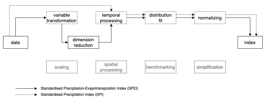
Figure 4.2 illustrates the pipeline steps of the two indexes. The two indexes are similar with the distinct that SPEI involves two additional steps – variable transformation and dimension reduction – prior to temporal processing. As introduced in Section 4.5, wrapper functions are available for both indexes as idx_spi() and idx_spei(), which allows for the specification of different time scales and distributions for fitting the aggregated series. In tidyindex, multiple indexes can be calculated collectively using the function compute_indexes(). Both SPI and SPEI are calculated across four time scales (6, 12, 24, and 36 months). The SPEI is fitted with two distributions (log-logistic and general extreme value distribution) and the gamma distribution is used for SPI:
# A tibble: 128,576 × 14
   .idx  .dist id               ym  prcp  tmax  tmin  tavg  long   lat
   <chr> <chr> <chr>         <mth> <dbl> <dbl> <dbl> <dbl> <dbl> <dbl>
 1 spei  gev   ASN000290… 1990 Jun   170  29.7  16.2  23.0  142. -15.5
 2 spei  gev   ASN000290… 1990 Jul   102  31.2  17.2  24.2  142. -15.5
 3 spei  gev   ASN000290… 1990 Aug     0  31.3  13.1  22.2  142. -15.5
 4 spei  gev   ASN000290… 1990 Sep     0  32.8  16.3  24.5  142. -15.5
 5 spei  gev   ASN000290… 1990 Oct     0  36.8  21.5  29.2  142. -15.5
 6 spei  gev   ASN000290… 1990 Nov   278  36.3  24.8  30.6  142. -15.5
 7 spei  gev   ASN000290… 1990 Dec  1869  34.4  24.5  29.4  142. -15.5
 8 spei  gev   ASN000290… 1990 Dec  1869  34.4  24.5  29.4  142. -15.5
 9 spei  gev   ASN000290… 1991 Jan  5088  31.2  24.4  27.8  142. -15.5
10 spei  gev   ASN000290… 1991 Jan  5088  31.2  24.4  27.8  142. -15.5
# ℹ 128,566 more rows
# ℹ 4 more variables: name <chr>, month <dbl>, .scale <dbl>,
#   .value <dbl>
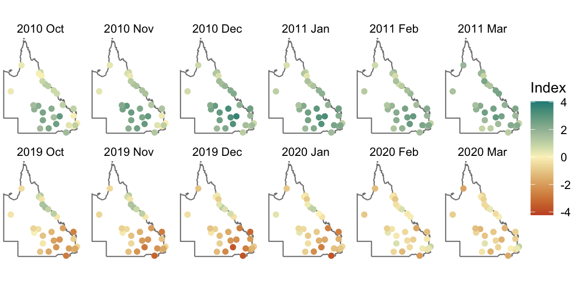
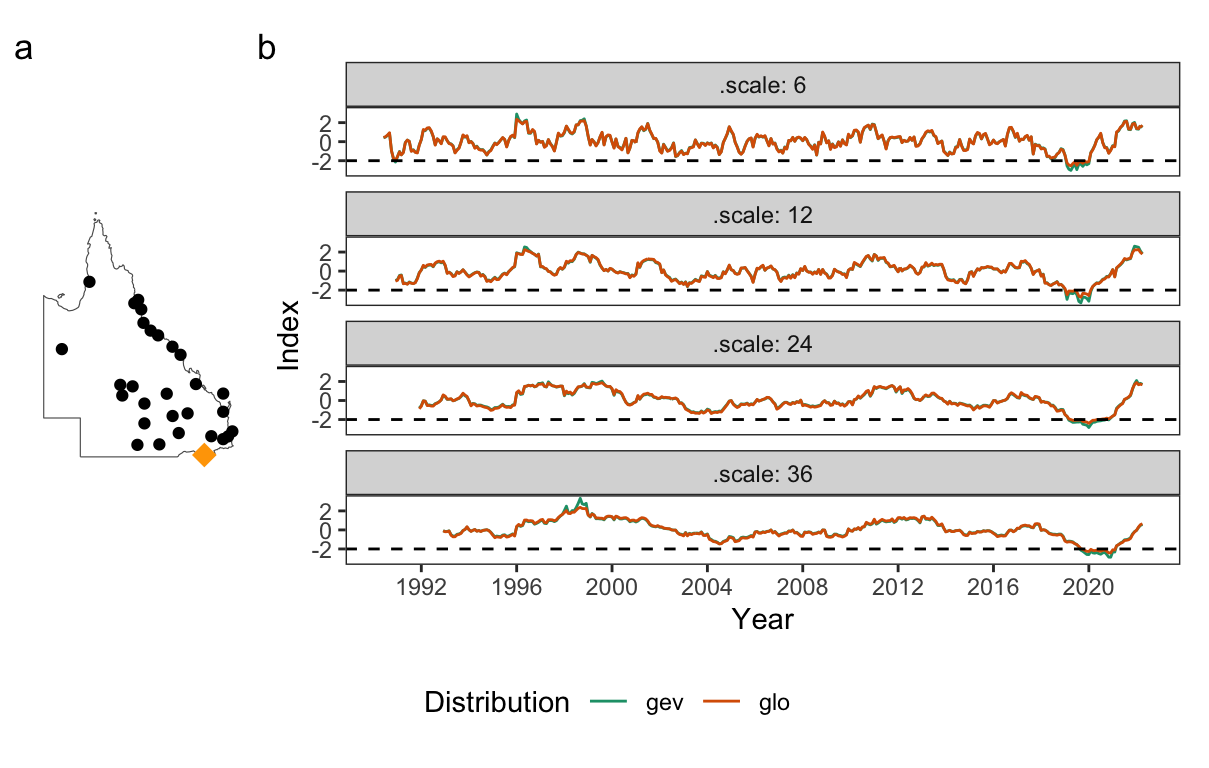
The output contains the original data, index values (.index), parameters used (.scale, .method, and .dist), and all the intermediate variables (pet, .agg, and .fitted). This data can be visualized to investigate the spatio-temporal distribution of the drought or flood events, as well as the response of index values to different time scales and distribution parameters at specific single locations. Figure 4.3 and Figure 4.4 exemplify two possibilities. Figure 4.3 presents the spatial distribution of SPI during two periods: October 2010 to March 2011 for the 2010/11 Queensland flood and October 2019 to March 2020 for the 2019 Australia drought, which contributes to the notorious 2019/20 bushfire season. Figure 4.4 displays the sensitivity of the SPEI series at the Texas post office to different time scales and fitted distributions. Larger time scales produce a smoother index across time, however, all time scales indicate an extreme drought (corresponding to -2 in SPEI) in 2020, confirming the severity of the drought across different time horizons. Moreover, the chosen distribution has less influence on the index, with general extreme value distribution tending to produce more extreme outcomes than log-logistic distribution for the extreme events (index > 2 or <-2).
Does a puff of change in variable weights cause a tornado in ranks?
The Global Gender Gap Index (GGGI), published annually by the World Economic Forum, measures gender parity by assessing relative gaps between men and women in four key areas: Economic Participation and Opportunity, Educational Attainment, Health and Survival, and Political Empowerment (World Economic Forum 2023). The index, defined on 14 variables measuring female-to-male ratios, first aggregates these variables into four dimensions (using the linear combination given by V-wgt in Table 4.1). The weights are the inverse of the standard deviation of each variable, scaled to sum to 1, thus ensuring equal relative contribution of each variable to each of the four new variables. These new variables are then combined through another linear combination (D-wgt in Table 4.1) to form the final index value. Figure 4.5 illustrates that the pipeline is constructed by applying the dimension reduction module twice on the data. The data for GGGI does not needs to be transformed or scaled so these steps are not included, but they might still need to be used for other similar indexes.

| Variable | V-wgt | Dimension | D-wgt | wgt |
|---|---|---|---|---|
| Labour force participation | 0.199 | Economy | 0.25 | 0.050 |
| Wage equality for similar work | 0.310 | 0.078 | ||
| Estimated earned income | 0.221 | 0.055 | ||
| Legislators senior officials and managers | 0.149 | 0.037 | ||
| Professional and technical workers | 0.121 | 0.030 | ||
| Literacy rate | 0.191 | Education | 0.25 | 0.048 |
| Enrolment in primary education | 0.459 | 0.115 | ||
| Enrolment in secondary education | 0.230 | 0.058 | ||
| Enrolment in tertiary education | 0.121 | 0.030 | ||
| Sex ratio at birth | 0.693 | Health | 0.25 | 0.173 |
| Healthy life expectancy | 0.307 | 0.077 | ||
| Women in parliament | 0.310 | Politics | 0.25 | 0.078 |
| Women in ministerial positions | 0.247 | 0.062 | ||
| Years with female head of state | 0.443 | 0.111 |
The 2023 GGGI data is available from the Global Gender Gap Report 2023 in the country’s economy profile and can be accessed in the tidyindex package as gggi with Table 4.1 as gggi_weights. The index can be reproduced with:
gggi %>%
  init(id = country) %>%
  add_meta(gggi_weights, var_col = variable) %>%
  dimension_reduction(
    index_new = aggregate_linear(
      ~labour_force_participation:years_with_female_head_of_state,
      weight = weight))
After initializing the gggi object and attaching the gggi_weights as meta-data, a single linear combination within the dimension reduction module is applied to the 14 variables (from column labour_force_participation to years_with_female_head_of_state), using the weight specified in the wgt column of the attached metadata. While computing the index from the original 14 variables, it remains unclear how the missing values are handled within the index, which impacts 68 out of the total 146 countries. However, after aggregating variables into the four dimensions, where no missing values exist, the index is reproducible for all the countries.
Figure 4.6 illustrates doing sensitivity analysis for GGGI, for a subset of 16 countries. Frame 12 shows the dot plot of the original index values sorted from highest to lowest. Leading the rankings are the Nordic countries (Iceland, Norway, and Finland) and New Zealand. The index values are between 0 and 1, and indicate proportional difference between men and women, with a value of 0.8 indicating women are 80% of the way to equality of these measures. There is a gap in values between these countries and the middle group (Brazil, Panama, Poland, Bangladesh, Kazakhstan, Armenia, and Slovakia), and another big drop to the next group (Pakistan, Iran, Algeria, and Chad). Afghanistan lags much further behind.
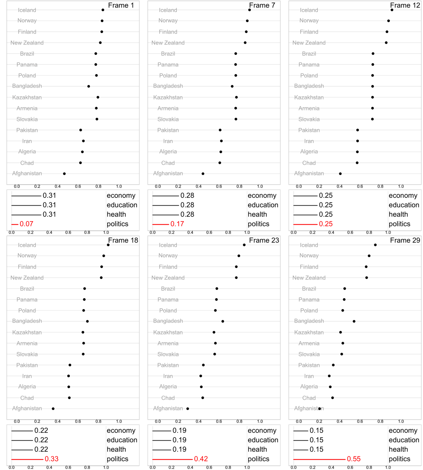
To make a simple illustration of sensitivity analysis, we slightly vary the weight for politics, between 0.07 and 0.52, while maintain equal weights among other dimensions. This can be viewed as an animation to examine change in relative index values as a response to the changing weights. This visualization technique, which presents a sequence of data projections, is referred to as a “tour” and the specific kind of tour used here to move between nearby projections is known as a “radial tour” (see Buja et al. (2005), Wickham et al. (2011), and Spyrison and Cook (2020) for more details).
Frames 1 and 6 show linear combinations where politics contributes less than the original. It is interesting to note that the gap between the Nordic countries and the middle countries dissipates, indicating that this component was one reason for the relatively higher GGGI values of these countries. Also interesting is the large drop in value for Bangladesh.
Frames 18, 24, 29 show linear combinations where politics contributes more than the original. The most notable feature is that Bangladesh retains it’s high index value whereas the other middle group countries decline, indicating that the politics score is a major component for Bangladesh’s index value.
Ideally, an index should be robust against minor changes in its construction components. This is not the case with GGGI, where small changes to one component lead to fairly large change in the index. The modular pipeline framework for computing the index makes it easy to conduct this type of sensitivity analysis, where one or more components are perturbed and the index re-calculated. One aspect of the GGGI not well-described in the Global Gender Gap Report is handling of missing values that are present in the initial variables for many countries, something that is common for this type of data. This could also be made more transparent with the dimension reduction module, by specifying an imputation method or providing warnings about missing values.
Decoding uncertainty through the wisdom of the crowd
Errors in measurement, variability and sampling error, may arise at various stages of the pipeline calculation, including from different parameterization choices, as illustrated from Section 4.6.1, or from the statistical summarization procedures applied in the pipeline. Although it may not be possible to perfectly measure these errors, it is important that they are recognised and estimated for an index, so that it is possible to compute confidence intervals. In this example, the Texas post office station highlighted in Figure 4.4 is used to illustrate one possibility to compute a confidence interval for the Standardized Precipitation Index (SPI). Bootstrapping is used to account for the sampling uncertainty in the distribution fit step of the index pipeline and to assess its impact on the SPI series.
In SPI, the distribution fit step fits the gamma distribution to the aggregated precipitation series separately for each month. This results in 32 or 33 points, from January 1990 to April 2022, for estimating each set of distribution parameters. To account for this sampling uncertainty with these samples, bootstrapping is used to generate replicates of the aggregated series. In the tidyindex package, this bootstrap sampling is activated when the argument .n_boot is set to a value other than the default of 1. In the following code, the Standardized Precipitation Index (SPI) is calculated using a time scale of 24. The bootstrap procedure samples the aggregated precipitation (.agg) for 100 iterations (.n_boot = 100) and then fits the gamma distribution. The resulting gamma probabilities are then transformed into normal densities in the normalizing step with normalise().
DATA |>
  temporal_aggregate(.agg = temporal_rolling_window(prcp, scale = 24)) |>
  distribution_fit(.fit = dist_gamma(var = ".agg", method = "lmoms",
                                     .n_boot = 100)) |>
  normalise(.index = norm_quantile(.fit))
The confidence interval can then be calculated using the quantile method from the bootstrap samples. Figure 4.7 presents the 80% and 95% confidence interval for the Texas post office station, in Queensland, Australia. From the start of 2019 to 2020, the majority of the confidence intervals lie below the extreme drought line (SPI = -2), suggesting a high level of certainty that the Texas post office is suffering from a drastic drought. The relatively wide confidence interval, as well as during the excessive precipitation events in 1996-1998 and 1999-2000, suggests a high variation of the gamma parameters estimated from the bootstrap samples and its difficulty to accurately quantify the drought and flood severity in extreme events.

4.7 Conclusion
The paper introduces a data pipeline comprising nine modules designed for the construction and analysis of indexes within the tidy framework. The pipeline offers a modular workflow to allow compute index with different parameterizations, to test minor changes to the original index definition, and to quantify uncertainties. The framework proposed in the paper is universal to index across diverse domains. Examples are provided, including the drought indexes (SPI and SPEI) and Global Gender Gap Index (GGGI), to demonstrate the index calculation with different time scales and distributions, to illustrate how slight adjustment of linear combination weights impact the index, and to calculate confidence intervals on the index.
4.8 Acknowledgement
This work is funded by a Commonwealth Scientific and Industrial Research Organisation (CSIRO) Data61 Scholarship. The article is created using Quarto (Allaire et al. 2022) in R (R Core Team 2021). The source code for reproducing this paper can be found at: https://github.com/huizezhang-sherry/paper-tidyindex.